Chapter 4 Task four : create sample distribution using bootsrapping

4.0.1 Bootstrapping :

The bootstrap method is a statistical technique for estimating quantities about a population by averaging estimates from multiple small data samples.

Importantly, samples are constructed by drawing observations from a large data sample one at a time and returning them to the data sample after they have been chosen. This allows a given observation to be included in a given small sample more than once. This approach to sampling is called sampling with replacement.

4.0.2 Example :

Bootstrapping in statistics, means sampling with replacement. So, if we have a group of individuals and , and want to bootstrap sample of ten individuals from this group , we could randomly sample any ten individuals but with bootsrapping, we are sampling with replacement so we could actually end up sampling 7 out of the ten individuals and three of the previously selected individuals might end up being sampled again.

set.seed(1234)
difference <- numeric()
size <- dim(df)[1]

for (i in 1:10000){
    sample_index <- sample(1:nrow(df), size = size, replace = TRUE)
    sample_df <- df[sample_index, ]
    controls_df <- sample_df[sample_df$group=="control",]
    experiments_df <- sample_df[sample_df$group=="experiment",]
    
    controls_ctr <- mean(ifelse(controls_df$action=="view and click", 1, 0))
    experiments_ctr <- mean(ifelse(experiments_df$action=="view and click", 1, 0))
    
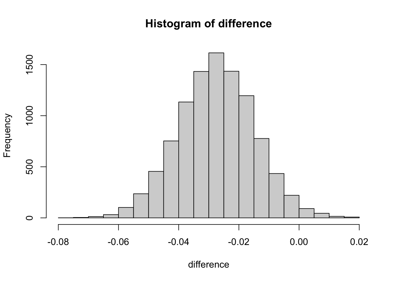
    difference <- append(difference, experiments_ctr - controls_ctr)
}

4.1 Task five : Evaluate the null hypothesis and draw conclustions.

The central limit theorem states that if you have a population with mean μ and standard deviation σ and take sufficiently large random samples from the population with replacement , then the distribution of the sample means will be approximately normally distributed.

hist(difference)

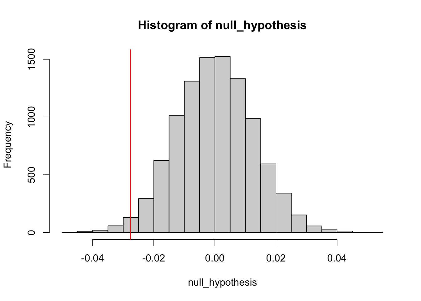
simulate the distribution under the null hypothesis (difference = 0)

null_hypothesis <- rnorm(n = length(difference), mean=0, sd=sd(difference))

hist(null_hypothesis)
abline(v= diff, col = "red")

The definition of a p-value is the probability of observing your statistic (or one more extreme in favor of the alternative) if the null hypothesis is true.

The confidence level is equivalent to 1 – the alpha level. So, if your significance level is 0.05, the corresponding confidence level is 95%.

i.e for P Value less than 0.05 we are 95% percent confident that we can reject the null hypothesis

compute p-value

mean((null_hypothesis > diff))

## [1] 0.9864

It says that we dont reject the null hypothesis. We can find more extreme values than our test statistics 98% of the time if the null hypothesis true.

4.2 alternative random sampling code

df %>%
    slice_sample(n = size, replace = T)

## # A tibble: 3,757 × 2
##    group      action
##    <chr>      <chr> 
##  1 experiment view  
##  2 experiment view  
##  3 experiment view  
##  4 control    view  
##  5 control    view  
##  6 control    view  
##  7 experiment view  
##  8 control    view  
##  9 experiment view  
## 10 control    view  
## # ℹ 3,747 more rows