Chapter 4 AB Testing
(Source)[https://matteocourthoud.github.io/post/synth/]
It is now widely accepted that the gold standard technique to compute the causal effect of a treatment (a drug, ad, product, …) on an outcome of interest (a disease, firm revenue, customer satisfaction, …) is AB testing, a.k.a. randomized experiments.
We randomly split a set of subjects (patients, users, customers, …) into a treatment and a control group and give the treatment to the treatment group. This procedure ensures that, ex-ante, the only expected difference between the two groups is caused by the treatment.
4.2 Concepts
Contamination:
One of the key assumptions in AB testing is that there is no contamination between treatment and control group.
Giving a drug to one patient in the treatment group does not affect the health of patients in the control group.
This might not be the case for example if we are trying to cure a contageous disease and the two groups are not isolated.
In the industry, frequent violations of the contamination assumption are network effects - my utility of using a social network increases as the number of friends on the network increases - and general equilibrium effects - if I improve one product, it might decrease the sales of another similar product.
Because of this reason, often experiments are carried out at a sufficiently large scale so that there is no contamination across groups, such as cities, states or even countries. Then another problem arises because of the larger scale: the treatment becomes more expensive. Giving a drug to 50% of patients in a hospital is much less expensive than giving a drug to 50% of cities in a country. Therefore, often only few units are treated but often over a longer period of time.
In these settings, a very powerful method emerged around 10 years age: Synthetic Control. The idea of synthetic control is to exploit the temporal variation in the data instead of the cross-sectional one (across time instead of across units).
This method is extremely popular in the industry - e.g. in companies like Google, Uber, Facebook, Microsoft, Amazon - because it is easy to interpret and deals with a setting that emerges often at large scales.
4.3 AI Summary
Studying A/B testing (also known as randomized controlled trials or RCTs) is a great way to understand experimental design in causal inference, particularly in contexts where random assignment is feasible and ethical considerations allow for manipulation of variables to observe their effects. Here’s a detailed overview to get you started:
4.3.1 A/B Testing (Randomized Controlled Trials)
A/B testing, or randomized controlled trials (RCTs), is an experimental design where participants or subjects are randomly assigned to different groups (treatment and control) to test the effectiveness of a particular intervention or treatment.
4.3.1.1 Key Concepts
- Random Assignment:
- Participants are assigned to either the treatment group (exposed to the intervention) or the control group (not exposed) through randomization. This helps ensure that any differences observed between the groups are due to the intervention rather than pre-existing differences.
- Controlled Environment:
- The experiment is conducted in a controlled environment where researchers can manipulate variables and minimize external influences that could affect the outcomes.
- Causal Inference:
- A/B testing allows researchers to make causal inferences about the effect of the intervention on the outcome variable. By comparing outcomes between the treatment and control groups, researchers can estimate the causal impact of the intervention.
4.3.1.2 Steps in A/B Testing
- Hypothesis Formulation:
- Define a clear hypothesis about the expected effect of the intervention on the outcome variable.
- Random Assignment:
- Randomly assign participants or subjects to the treatment and control groups. Randomization helps ensure that the groups are comparable on average, reducing the risk of bias.
- Implementation of Intervention:
- Implement the intervention or treatment with the treatment group while keeping conditions unchanged for the control group.
- Outcome Measurement:
- Measure the outcome of interest for both the treatment and control groups after the intervention. This could be metrics like conversion rates, satisfaction scores, or health outcomes.
- Statistical Analysis:
- Compare the outcomes between the treatment and control groups using statistical methods (e.g., t-tests, regression analysis) to determine if there is a significant difference attributable to the intervention.
- Interpretation of Results:
- Interpret the results to determine whether the intervention had a causal effect on the outcome variable. Consider factors such as statistical significance, effect size, and practical significance.
4.3.1.3 Advantages of A/B Testing
Causal Inference: Allows for strong causal claims about the impact of interventions.
Control Over Variables: Researchers have control over experimental conditions, minimizing confounding factors.
Versatility: Applicable across various fields including marketing, healthcare, education, and technology.
4.3.1.4 Example Application
Imagine a company wants to test the effectiveness of two different website layouts (A and B) on user engagement:
Hypothesis: Layout B will lead to higher user engagement compared to Layout A.
Random Assignment: Users visiting the website are randomly assigned to either see Layout A or Layout B.
Outcome Measurement: Engagement metrics such as click-through rates or time spent on the website are measured for both groups.
Analysis: Statistical tests are conducted to compare engagement metrics between Layout A and Layout B.
Conclusion: If Layout B shows significantly higher engagement metrics, the company may decide to implement Layout B on their website.
4.3.2 Concepts:
4.3.2.1 Effect Size
Definition: Effect size quantifies the magnitude of the difference or relationship between variables in a study. It provides a standardized measure of the strength of an effect or phenomenon being studied, independent of sample size.
Key Points:
Standardized Measure: Effect size is expressed in standard deviation units or other standardized metrics, making it comparable across different studies.
Interpretation: A larger effect size indicates a stronger relationship or more substantial difference between groups or conditions.
Example: In an A/B test measuring website conversion rates:
- If Group A (control) has a conversion rate of 5% and Group B (treatment) has a conversion rate of 7%, the effect size could be quantified using metrics like Cohen’s d or relative risk increase to indicate the practical significance of the difference.
Certainly! Cohen’s d and relative risk are commonly used effect size measures in different contexts, providing standardized ways to quantify and compare the magnitude of effects between groups or conditions in research studies. Here’s an explanation of each:
4.3.2.2 Cohen’s d
Definition: Cohen’s d is a standardized measure of effect size that indicates the difference between two means (e.g., treatment group mean and control group mean) in terms of standard deviation units.
Formula: $ d = $
where: - $ {X}_1$ and ${X}_2 $ are the means of the two groups, - $ s $ is the pooled standard deviation of the two groups.
Interpretation: - Effect Size Magnitude: Cohen’s d values are interpreted as follows: - Small effect: d = 0.2 - Medium effect: d = 0.5 - Large effect: d = 0.8
Example: In a study comparing the effectiveness of two teaching methods on exam scores: - If the mean exam score in Method A (treatment) is 80 and in Method B (control) is 75, and the pooled standard deviation is 10, then Cohen’s d would be \(\frac{80 - 75}{10} = 0.5\), indicating a medium effect size.
4.3.2.3 Relative Risk
Definition: Relative risk (RR) is a measure of the strength of association between a risk factor (or exposure) and an outcome in epidemiology and medical research. It compares the risk of an outcome occurring in the exposed group versus the unexposed (or control) group.
Formula: \[ RR = \frac{\text{Risk in exposed group}}{\text{Risk in unexposed group}} \]
Interpretation: - RR = 1: Indicates no association between exposure and outcome. - RR > 1: Indicates higher risk in the exposed group compared to the unexposed group. - RR < 1: Indicates lower risk in the exposed group compared to the unexposed group.
Example: In a clinical trial evaluating a new drug for heart disease: - If the risk of heart attack among patients taking the new drug is 10% and among patients not taking the drug (control group) is 20%, then the relative risk would be \(\frac{0.10}{0.20} = 0.5\). - This means patients taking the drug have half the risk of experiencing a heart attack compared to those not taking the drug.
4.3.3 Comparison and Usage
Cohen’s d: Typically used in studies comparing means of continuous variables (e.g., exam scores, reaction times) between two groups.
Relative Risk: Primarily used in studies of binary outcomes (e.g., disease incidence, event occurrence) to compare the risk of an outcome between exposed and unexposed groups.
Both measures provide valuable insights into the strength and direction of effects in research studies. The choice between Cohen’s d and relative risk depends on the nature of the data (continuous or binary) and the specific research question being addressed. Researchers often use these effect size measures alongside significance testing to provide a comprehensive assessment of the findings’ practical and statistical significance.
4.3.4 Significance
Definition: Statistical significance determines whether the observed results in a study are likely to be due to the intervention (or other factors being studied) rather than random chance. It is typically assessed through hypothesis testing.
Key Points: - Hypothesis Testing: Statistical tests (e.g., t-tests, ANOVA, chi-square tests) evaluate whether the observed differences between groups are statistically significant.
Threshold: Results are deemed statistically significant if the probability (p-value) of observing such differences due to chance alone is below a predefined significance level (commonly set at 0.05).
Does Not Equal Importance: Statistical significance does not necessarily equate to practical or clinical significance; it only indicates the reliability of the observed effect.
Example: In a clinical trial evaluating a new drug: - If the treatment group shows a significantly lower incidence of adverse effects compared to the control group (p < 0.05), it suggests that the drug may have a beneficial effect on reducing adverse reactions.
4.3.5 Group Size
Definition: Group size refers to the number of participants or subjects included in each experimental group or condition in a study. It directly influences the statistical power and precision of the study’s results.
Key Points: - Statistical Power: Larger group sizes generally increase the statistical power of a study, making it more likely to detect a true effect if one exists. - Precision: Larger group sizes reduce sampling variability and increase the precision of estimates (e.g., mean values, effect sizes). - Resource Allocation: Group size is often determined by practical considerations such as budget, time constraints, ethical considerations, and expected effect size.
Example: In an A/B test comparing two marketing strategies: - If Group A consists of 1000 customers and Group B consists of 500 customers, the study’s power to detect differences between the groups will be influenced by the unequal group sizes.
4.3.6 Relationship Between Effect Size, Significance, and Group Size
- Effect Size and Significance: A larger effect size increases the likelihood of achieving statistical significance with smaller group sizes. Conversely, smaller effect sizes may require larger group sizes to achieve statistical significance.
- Group Size and Precision: Larger group sizes generally provide more precise estimates of effects and reduce the impact of random variability in the data.
- Balancing Factors: Researchers often balance effect size, significance level, and group size to achieve meaningful and reliable results within practical constraints.
4.3.7 Conclusion
Understanding effect size, significance, and group size is crucial for interpreting and evaluating research findings accurately. Effect size measures the magnitude of effects, significance assesses the likelihood of results being due to chance, and group size influences the study’s statistical power and precision. Together, these concepts help researchers draw meaningful conclusions and inform decision-making based on empirical evidence.
4.3.7.1 Baseline conversion rate
The baseline conversion rate is the current conversion rate for the page you are testing. Conversion rate is the number of conversions divided by the total number of visitors.
4.3.7.2 Minimum detectable effect (MDE)
After baseline conversion rate, you need to decide how much change from the baseline (how big or small a lift) you want to detect. You wil need less traffic to detect big changes and more traffic to detect small changes.
To demonstrate, let us use an example with a 20% baseline conversion rate and a 5% MDE. Based on these values, your experiment will be able to detect 80% of the time when a variation’s underlying conversion rate is actually 19% or 21% (20%, +/- 5% × 20%). If you try to detect differences smaller than 5%, your test is considered underpowered.
Power is a measure of how well you can distinguish the difference you are detecting from no difference at all. So running an underpowered test is the equivalent of not being able to strongly declare whether your variations are winning or losing.
4.4 Size of the Control Group
Calculating the appropriate size of the control group in an experiment involves several important factors to ensure the study has sufficient power to detect a true effect if one exists. Here are the key factors that influence control group size calculation:
- Effect Size (δ)
Effect size is a measure of the magnitude of the difference between groups or the strength of the relationship between variables. It quantifies the practical significance of the treatment effect.
Influence on Sample Size:
- A larger effect size requires a smaller sample size to detect a significant difference.
- A smaller effect size requires a larger sample size to achieve the same level of power.
- Significance Level (α)
The significance level (α) is the threshold for determining whether the observed effect is statistically significant. It represents the probability of committing a Type I error (rejecting a true null hypothesis).
Common Values: - α is typically set at 0.05, meaning there is a 5% chance of rejecting the null hypothesis when it is true.
Influence on Sample Size:
A lower α (e.g., 0.01) requires a larger sample size to maintain the same power, as the test becomes more stringent.
A higher α (e.g., 0.10) allows for a smaller sample size but increases the risk of Type I errors.
- Power (1 - β)
Power is the probability of correctly rejecting a false null hypothesis. It reflects the study’s ability to detect an effect if one exists.
Common Values: - A common target for power is 0.80, indicating an 80% chance of detecting a true effect.
Influence on Sample Size: - Higher power (e.g., 0.90) requires a larger sample size. - Lower power (e.g., 0.70) allows for a smaller sample size but increases the risk of Type II errors (failing to detect a true effect).
- Variability (σ)
Variability refers to the spread or dispersion of data points within a population, often measured by the standard deviation (σ).
Influence on Sample Size: - Higher variability (greater standard deviation) requires a larger sample size to detect a significant difference. - Lower variability allows for a smaller sample size as the effect is easier to detect against a less noisy background.
- Allocation Ratio
Definition: The allocation ratio determines the proportion of participants assigned to the treatment group versus the control group. An equal allocation ratio (1:1) means equal numbers in both groups.
Influence on Sample Size: - Unequal allocation ratios (e.g., 2:1 or 3:1) may be used based on study design or practical considerations but can affect the total sample size required to achieve the desired power. - An equal allocation ratio generally provides the most statistically efficient design, minimizing the total sample size required.
- Dropout Rate
Definition: The dropout rate accounts for participants who may leave the study before its completion, affecting the effective sample size.
Influence on Sample Size: - Anticipated dropouts should be factored into the initial sample size calculation to ensure the study retains adequate power despite participant loss.
4.4.1 Sample Size Calculation Formula
For comparing two means, the sample size for each group can be calculated using:
\[ n = \left( \frac{(Z_{\alpha/2} + Z_{\beta}) \cdot \sigma}{\delta} \right)^2 \]
where: - \(n\) is the sample size per group, - \(Z_{\alpha/2}\) is the critical value for the desired significance level, - \(Z_{\beta}\) is the critical value for the desired power, - \(\sigma\) is the standard deviation, - \(\delta\) is the effect size.
4.4.2 Conclusion
Determining the control group size involves considering the desired effect size, significance level, power, variability in the data, allocation ratio, and potential dropout rates. Properly calculating the control group size ensures that the study is adequately powered to detect meaningful effects, thereby enhancing the validity and reliability of the research findings.
4.4.3 Statistical Assumptions for Randomized Controlled Trials (RCTs)
Randomized Controlled Trials (RCTs) are considered the gold standard in experimental research due to their ability to minimize bias and establish causality. However, the validity of RCT results depends on several key statistical assumptions:
Randomization:
- Assumption: Participants are randomly assigned to treatment and control groups.
- Purpose: Ensures that the groups are comparable on average, reducing selection bias and balancing both known and unknown confounders.
Independence:
- Assumption: Observations are independent of each other.
- Purpose: Ensures that the outcome of one participant does not influence the outcome of another, which is crucial for valid statistical inference.
Consistency:
- Assumption: The treatment effect is consistent across all participants.
- Purpose: Ensures that the treatment effect observed in the sample can be generalized to the broader population.
Exclusion of Confounders:
- Assumption: No confounding variables influence the treatment-outcome relationship.
- Purpose: Ensures that the observed effect is due to the treatment and not due to other external factors.
Stable Unit Treatment Value Assumption (SUTVA):
- Assumption: The potential outcomes for any participant are not affected by the treatment assignment of other participants.
- Purpose: Prevents interference between participants, ensuring that each participant’s outcome is solely a result of their treatment assignment.
No Systematic Differences in Measurement:
- Assumption: Measurement of outcomes is consistent and unbiased across treatment and control groups.
- Purpose: Ensures that outcome measures are not systematically biased by the treatment assignment.
4.4.4 Robustness Checks
Robustness checks involve testing the stability and reliability of the study’s findings under various assumptions and conditions. They help to confirm that the results are not sensitive to specific assumptions or potential biases. Key robustness checks for RCTs include:
- Sensitivity Analysis:
- Purpose: Evaluates how the results change with different assumptions or parameters.
- Method: Adjusting key assumptions or parameters (e.g., different definitions of the outcome variable) to see if the results remain consistent.
- Subgroup Analysis:
- Purpose: Examines the effect of the treatment within different subgroups of the sample.
- Method: Dividing the sample into subgroups (e.g., by age, gender, or baseline risk) and checking if the treatment effect is consistent across these groups.
- Placebo Tests:
- Purpose: Tests whether the results hold when using a placebo treatment.
- Method: Using a placebo group to confirm that the observed effects are specifically due to the treatment and not to other factors.
- Alternative Specifications:
- Purpose: Tests the robustness of the results to different model specifications.
- Method: Using alternative statistical models or different functional forms to ensure results are not model-dependent.
- Attrition Analysis:
- Purpose: Examines the impact of participant dropout on the study results.
- Method: Analyzing the characteristics of dropouts and conducting analyses to understand if and how attrition might bias the results.
4.4.5 Validation Methods
Validation methods are used to confirm the internal and external validity of the study’s findings. These methods help to ensure that the results are credible and can be generalized to other settings or populations.
- Internal Validity Checks:
- Balance Checks:
- Purpose: Ensures that randomization created comparable groups.
- Method: Comparing baseline characteristics between treatment and control groups to check for balance.
- Compliance Checks:
- Purpose: Ensures participants adhere to the assigned treatment.
- Method: Analyzing adherence rates and conducting per-protocol analyses if necessary.
- Balance Checks:
- External Validity Checks:
- Population Representativeness:
- Purpose: Ensures that the study sample is representative of the broader population.
- Method: Comparing sample characteristics to the target population and discussing potential generalizability limitations.
- Replication Studies:
- Purpose: Confirms the findings by replicating the study in different settings or with different populations.
- Method: Conducting similar studies in various contexts to see if the results hold.
- Population Representativeness:
- Model Validation:
- Cross-Validation:
- Purpose: Assesses the predictive accuracy of the statistical model.
- Method: Using techniques like k-fold cross-validation to test the model’s performance on different subsets of the data.
- Out-of-Sample Validation:
- Purpose: Ensures the model performs well on new, unseen data.
- Method: Validating the model on a separate dataset that was not used for model training.
- Cross-Validation:
4.4.6 Conclusion
The validity of RCT findings hinges on several key assumptions, and the credibility of these results is reinforced through robustness checks and validation methods. Robustness checks test the stability of findings under different conditions, while validation methods confirm the internal and external validity of the results, ensuring they are generalizable and reliable. Understanding and addressing these factors is crucial for conducting and interpreting high-quality research.
4.5 Example: Conversion Rate of an E-Commerce Website
Suppose an e-commerce website wants to test if implementing a new feature (e.g., layout or button) will significantly improve conversion rate.
conversion rate: number of purchases divided by number of sessions/visits
We can randomly show the new webpage to 50% of the users. Then, we have a test group and a control group. Once we have enough data points, we can test if the conversion rate in the treatment group is significantly higher (one side test) than that in the control group.
The null hypothesis is that conversion rates are not significantly different in the two group.
Sample Size for Comparing Two Means.
One way to perform the test is to calculate daily conversion rates for both the treatment and the control groups.
Since the conversion rate in a group on a certain day represents a single data point, the sample size is actually the number of days.
Thus, we will be testing the difference between the mean of daily conversion rates in each group across the testing period. The formula for estimate minimum sample size is as follows:
Sample Size Estimate for A/B Test
In an A/B test, the sample size (\(n\)) required for each group can be estimated using the formula:
\[n = \frac{{2 \cdot (Z_{\alpha/2} + Z_{\beta})^2 \cdot \sigma^2}}{{\delta^2}}\]
where: $ n : $ $ Z_{/2} : $ $ Z_{} : $ $ ^2 : $ $ : $
This formula helps in determining the sample size needed to achieve desired levels of significance and power in an A/B test.
For our example, let’s assume that the mean daily conversion rate for the past 6 months is 0.15 and the sample standard deviation is 0.05.
With the new feature, we expect to see a 3% absolute increase in conversion rate. Thus, for the conversion rate for the treatment group will be 0.18. We also assume that the sample standard deviations are the same for the two group.
Our parameters are as follows.
\(\mu_1 = 0.15\) \(\mu_2 = 0.18\) \(\sigma_1 = \sigma_2 = 0.05\)
Assuming \(\alpha = 0.05\) and \(\beta = 0.20\) (\(power = 0.80\)), applying the formula, the required minimum sample size is 35 days.
This is consistent with the result from this web calculator.
Sample Size for Comparing Two Proportions
The two-means approach considers each day+group as a data point. But what if we focus on individual users and visits?
What if we want to know how many visits/sessions are required for the testing? In this case, the conversion rate for a group is basically all purchases divided by all sessions in that group. If each session is a Bernoulli trial (convert or not), each group follows a binomial distribution.
To test the difference in conversion rate between the treatment and control groups, we need a test of two proportions. The formula for estimating the minimum required sample size is as follows.
Summary: Sample Size Estimate for Comparing Proportions
When comparing proportions in two independent groups, the sample size (\(n\)) required for each group can be estimated using the formula:
\[n = \frac{{2 \cdot (Z_{\alpha/2} + Z_{\beta})^2 \cdot (p(1-p))}}{{\delta^2}}\]
where:
\(n : \text{ Sample size per group}\)
\(Z_{\alpha/2} : \text{ Critical value for significance level}\)
\(Z_{\beta} : \text{ Critical value for desired power}\)
\(p : \text{ Expected proportion in one group}\)
\(\delta : \text{ Minimum detectable difference in proportions}\)
This formula helps in determining the sample size needed to detect a specified difference in proportions between two groups with desired levels of significance and power.
Assuming 50–50 split, we have the following parameters:
\(p_1 = 0.15\)
\(p_2 = 0.18\)
\(k = 1\)
Using \(\alpha = 0.05\) and \(\beta = 0.20\), applying the formula, the required sample size is \(1,892\) sessions per group.
4.6 Example: A/B Test
A/B testing is an experiment where two or more variants are evaluated using statistical analysis to determine which variation performs better for a given conversion goal.
A/B testing is widely used by digital marketing agencies as it is the most effective method to determine the best content for converting visits into sign-ups and purchases.
In this scenario, you will set up hypothesis testing to advise a digital marketing agency on whether to adopt a new ad they designed for their client.
Assume you are hired by a digital marketing agency to conduct an A/B test on a new ad hosted on a website. Your task is to determine whether the new ad outperforms the existing one.
The agency has run an experiment where one group of users was shown the new ad design, while another group was shown the old ad design. The users’ interactions with the ads were observed, specifically whether they clicked on the ad or not.
4.6.1 Task 1: Load the data
In this task, we will import our libraries and then load our dataset
## ── Attaching core tidyverse packages ───────────── tidyverse 2.0.0 ──
## ✔ dplyr     1.1.2     ✔ readr     2.1.4
## ✔ forcats   1.0.0     ✔ stringr   1.5.0
## ✔ ggplot2   3.4.4     ✔ tibble    3.2.1
## ✔ lubridate 1.9.3     ✔ tidyr     1.3.0
## ✔ purrr     1.0.1
## ── Conflicts ─────────────────────────────── tidyverse_conflicts() ──
## ✖ dplyr::filter() masks stats::filter()
## ✖ dplyr::lag()    masks stats::lag()
## ℹ Use the conflicted package (<http://conflicted.r-lib.org/>) to force all conflicts to become errorslibrary(readxl)
df <- read_excel('/Users/deayan/Desktop/GITHUB/10_Causal_Notes/__repo/data/AB_Test.xlsx')## Rows: 3,757
## Columns: 2
## $ group <chr> "experiment", "control", "control", "control", "control", "cont…
## $ action <chr> "view", "view", "view and click", "view and click", "view", "vi…## # A tibble: 4 × 3
## group action n
## <chr> <chr> <int>
## 1 control view 1513
## 2 control view and click 363
## 3 experiment view 1569
## 4 experiment view and click 3124.6.2 Task 2: Set up Hypothesis
experiment group: the group that is involved in the new experiment . i.e the group that received the new ad .
Control group: the 2nd group that didn’t receive the new ad
Click-through rate (CTR): the number of clicks advertisers receive on their ads per number of impressions.
##
##    control experiment
## 1876 1881## # A tibble: 2 × 2
## group n
## <chr> <int>
## 1 control 1876
## 2 experiment 1881## action
## group view view and click
## control 1513 363
## experiment 1569 312## action
## group view view and click
## control 0.8065032 0.1934968
## experiment 0.8341308 0.1658692## # A tibble: 2 × 3
## group n prop
## <chr> <int> <dbl>
## 1 control 1876 0.499
## 2 experiment 1881 0.501x <- df %>%
group_by(group, action)%>%
summarise(n = n(), .groups = 'drop')%>%
pivot_wider(names_from = action, values_from = n, values_fill = list(n = 0))
names(x) <- c("group", "view", "view_click")
x%>%
group_by(group)%>%
transmute(view1 = view/(view+view_click),
view_click1 = view_click/(view+view_click))## # A tibble: 2 × 3
## # Groups: group [2]
## group view1 view_click1
## <chr> <dbl> <dbl>
## 1 control 0.807 0.193
## 2 experiment 0.834 0.166The null hypothesis is what we assume to be true before we collect the data, and the alternative hypothesis is usually what we want to try and prove to be true.
So in our experiment than null hypothesis is assuming that the old ad is better than than new one.
Then we set the significance level \(\alpha\).
The significance level is the probability of rejecting the null hypothesis when it’s true. (Type I error rate)
For example, a significance level of 0.05 indicates a 5% risk of concluding that a difference exists when there is no actual difference.
Lower significance levels indicate that you require stronger evidence before you reject the null hypothesis.
So we will set our significance level to be 0.05. And if we reject the null hypothesis as a result of our experiment, then by having significant level of 0.05 then we are 95% confident that we can reject the null hypothesis.
So setting the significance level is about how confident you are while you reject the null hypothesis, the fourth step is calculating the corresponding P value.
The definition of P value is the probability of observing your statistic, if the null hypothesis is true. And then we will draw a conclusion whether to go for the new ad or not.
Hypothesis Testing steps:
1) Specify the Null Hypothesis.
2) Specify the Alternative Hypothesis.
3) Set the Significance Level (a)
4) Calculate the Corresponding P-Value.
5) Drawing a Conclusion
Our Hypothesis
Hypothesis is that the click through rate associated with the new ad is less than that associated with the old ad, which means that the old ad is better than than new one.
And the alternative hypothesis will be the opposite.
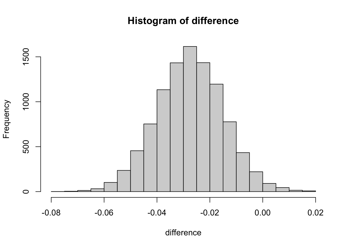
4.6.3 Task 3: Compute the difference in the click-through rate
This task we will compute the difference in the click through rate between the control and experiment groups.
control_ctr <-
    mean(ifelse(control_df$action=="view and click", 1, 0))

experiment_ctr <-
    mean(ifelse(experiment_df$action=="view and click", 1, 0))

diff <- experiment_ctr - control_ctr
diff
## [1] -0.027627584.6.4 Task four : create sample distribution using bootsrapping
4.6.4.1 Bootstrapping :
The bootstrap method is a statistical technique for estimating quantities about a population by averaging estimates from multiple small data samples.
Importantly, samples are constructed by drawing observations from a large data sample one at a time and returning them to the data sample after they have been chosen. This allows a given observation to be included in a given small sample more than once. This approach to sampling is called sampling with replacement.
4.6.4.2 Example :
Bootstrapping in statistics, means sampling with replacement. So, if we have a group of individuals and , and want to bootstrap sample of ten individuals from this group , we could randomly sample any ten individuals but with bootsrapping, we are sampling with replacement so we could actually end up sampling 7 out of the ten individuals and three of the previously selected individuals might end up being sampled again.
set.seed(1234)
difference <- numeric()
size <- dim(df)[1]

for (i in 1:10000){
    sample_index <- sample(1:nrow(df), size = size, replace = TRUE)
    sample_df <- df[sample_index, ]
    controls_df <- sample_df[sample_df$group=="control",]
    experiments_df <- sample_df[sample_df$group=="experiment",]

    controls_ctr <- mean(ifelse(controls_df$action=="view and click", 1, 0))
    experiments_ctr <- mean(ifelse(experiments_df$action=="view and click", 1, 0))

    difference <- append(difference, experiments_ctr - controls_ctr)
}
4.6.5 Task five : Evaluate the null hypothesis and draw conclustions.
The central limit theorem states that if you have a population with mean μ and standard deviation σ and take sufficiently large random samples from the population with replacement , then the distribution of the sample means will be approximately normally distributed.
simulate the distribution under the null hypothesis (difference = 0)
null_hypothesis <- rnorm(n = length(difference), mean=0, sd=sd(difference))

hist(null_hypothesis)
abline(v= diff, col = "red")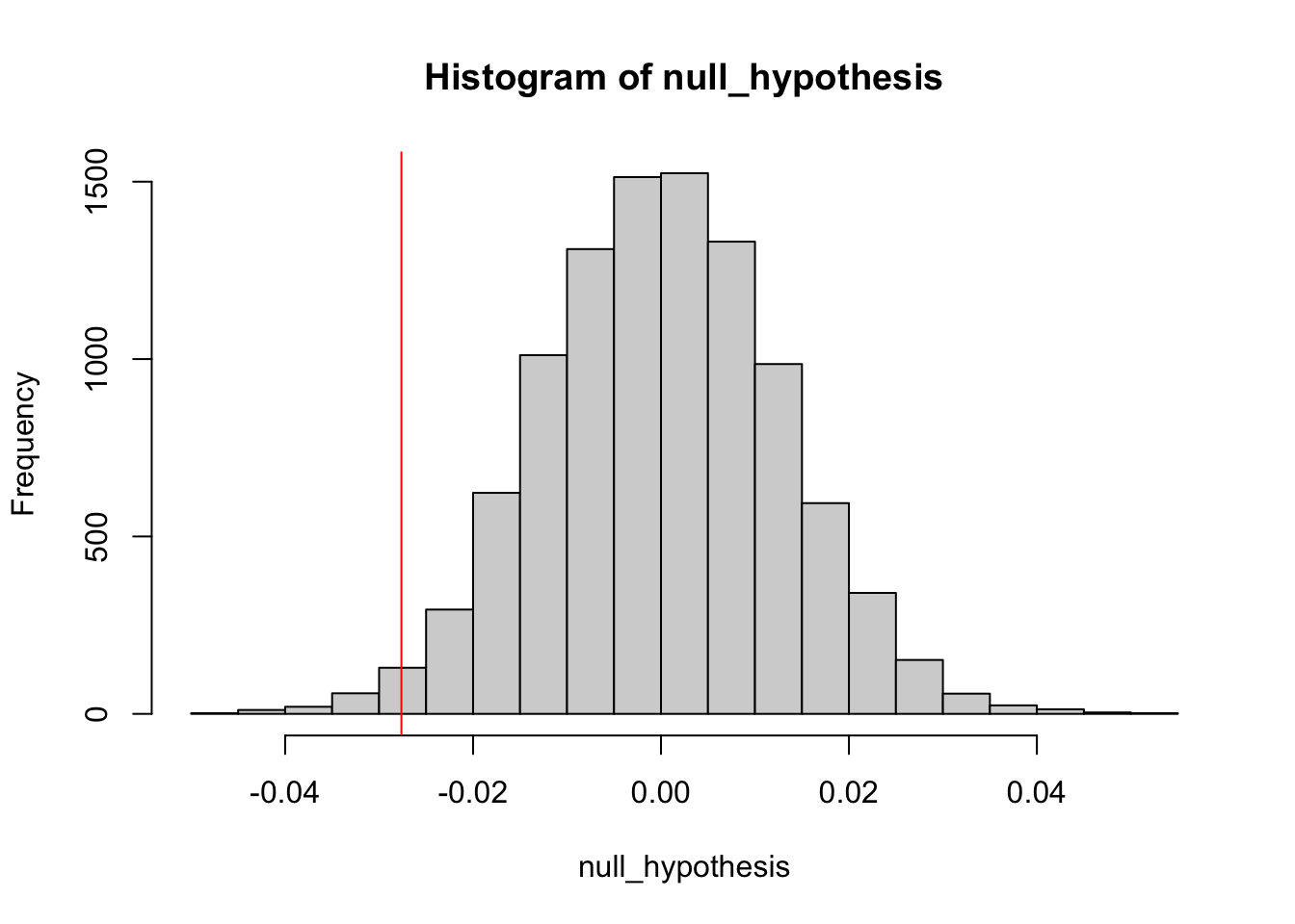
The definition of a p-value is the probability of observing your statistic (or one more extreme in favor of the alternative) if the null hypothesis is true.
The confidence level is equivalent to 1 – the alpha level. So, if your significance level is 0.05, the corresponding confidence level is 95%.
i.e for P Value less than 0.05 we are 95% percent confident that we can reject the null hypothesis
compute p-value
## [1] 0.9864It says that we dont reject the null hypothesis. We can find more extreme values than our test statistics 98% of the time if the null hypothesis true.